Lecture 1: R Basics & the Tidyverse
Setting our working directory
The working directory is a really powerful concept in R – it is where R saves any output files you create during an analysis and it is the place where R looks for any data you want to read in. When you installed R & RStudio in Lecture 0, we asked you to create a folder on your Desktop called Moneyball. This will be your working directory for the duration of the course.
Every time you open RStudio, it automatically sets the working
directory to some default folder on your computer. To see what that is,
we’ll open RStudio and look at the console pane. We can also check our
working directory with the code getwd()
Once we open RStudio, before we do anything, we need to tell R to change the working directory to our Moneyball folder. We can do this in a couple of ways:
- In the top toolbar, Session/Set Working Directory/Choose Working
Directory allows us to select and set our working directory from our
files.
- The code
setwd("~/Desktop/Moneyball")sets our working directory to the Moneyball folder, and can be edited for any file location.
Important: for the next three weeks, every time you open up RStudio, the first thing you should do is set your working directory to the Moneyball folder.
Base R
Now that we have set our working directory, we can work with data.
The basic functionality included with R is called Base R. Simple
arithmetic such as 2*3 and mean(3:9) are
included as initial functionality in base R. We can also assign values
to vectors and plot graphs.
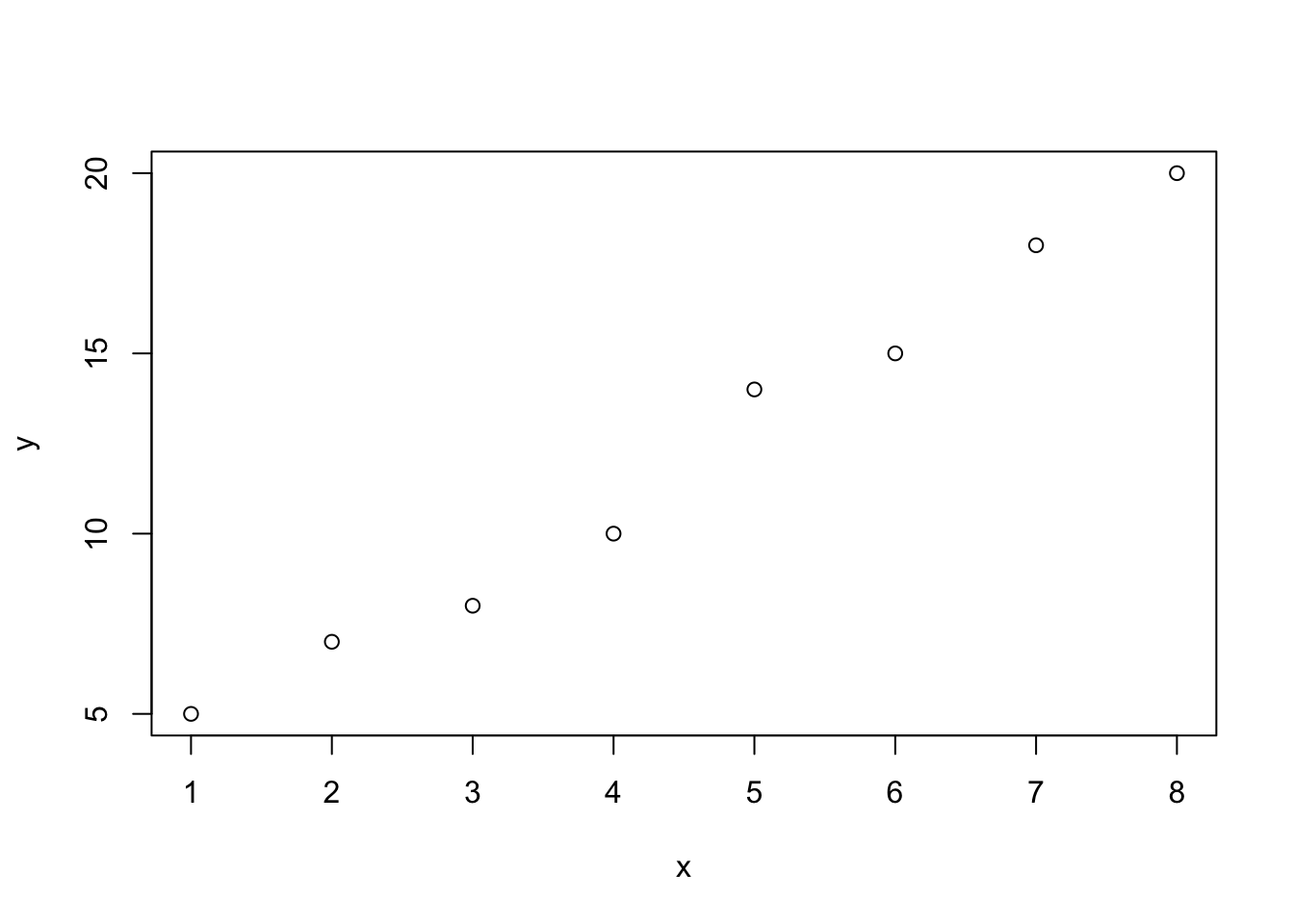 In the above code, we assigned the numbers 1-8 to x and assigned the
numbers 5, 7, …, 18, 20 to y. Then we plotted the graph with x and y, as
if they were coordinate points.
In the above code, we assigned the numbers 1-8 to x and assigned the
numbers 5, 7, …, 18, 20 to y. Then we plotted the graph with x and y, as
if they were coordinate points.
We did all that with Base R. However, the functionality provided by a fresh install of R is only a small fraction of the computing power available with R. Extra functionality comes from add-ons, or packages, created by developers.
Packages
So far we have seen only the most basic of R’s functionality. Arguably, one of the things that makes R so powerful is the ease with which users are able to define their own functions and release them to the public.As Hadley Wickham defines them, “[R] packages are fundamental units of reproducible code. They include reusable R functions, the documentation that describes how to use them, and sample data.” As of June 18, 2020, there are 15,805 packages available from the Comprehensive R Archive Network (CRAN). The scope of these packages is vast: there are some designed for scraping data from the web, pre-processing data to get it into an analyzable format, performing standard and specialized statistical analyses, and to publish your results. People have also released packages tailored to very specific applications like analyzing baseball data. There are also some more whimsical packages, like one that allow you to display your favorite XKCD comic strip!
We can install packages in several ways:
In the top toolbar, Tools/Install Packages allows us to search and install packages to our library.
In the bottom right pane, the Packages tab has an install button. After clicking this button, we can search for and install a package and its dependencies (for now, always leave the ‘Install dependencies’ box checked).
The code
install.packages("tidyverse")will install tidyverse, or any other package.
After installing a package, we have to load the package before using it. Again, we have two options for loading a package:
- In bottom right pane, the Packages tab allows us to search and
scroll for packages. The checkbox to the left of the package name
indicates if the package is loaded. By checking that box, we can load
the package.
- The code
library(tidyverse)will load tidyverse, or any other package.
The tidyverse
For the rest of the course, we will be working within the tidyverse, which consists of several R packages for data manipulation, exploration, and visualization. They are all based on a common design philosophy, mostly developed by Hadley Wickham (whose name you will encounter a lot as you gain more experience with R).
To access tidyverse, first we first need to install the tidyverse package:
The install.packages() function is one way of installing
packages in R. You can also use Tools/Install Packages or click on the
Packages tab in the bottom right pane of your RStudio view and then
click on Install to type in the package you want to install.
Now with the tidyverse suite of packages installed, we
can load them with the following code:
When you do that, you’ll see a lot of output to the console, most of
which you can safely ignore for now. Note you only need to
install the package once. However, each time you open up a new R session
and want to use the tidyverse, you will need to run line
library(tidyverse) at the start.
Reading in tabular data
Almost all of the data we will encounter in this course (and in the real world) will be tabular. Each row will represent a separate observation and each column will record a particular measurement. For instance, the table below lists different statistics for several basketball players from the 2015-16 NBA regular season. The statistics are: field goal makes (FGM), field goal attempts (FGA), three point makes (TPM), three point attempts (TPA), free throw makes (FTM), and free throw attempts (FTA).
| PLAYER | SEASON | FGM | FGA | TPM | TPA | FTM | FTA |
|---|---|---|---|---|---|---|---|
| Stephen Curry | 2016 | 805 | 1597 | 402 | 887 | 363 | 400 |
| Damian Lillard | 2016 | 618 | 1474 | 229 | 610 | 414 | 464 |
| Jimmy Butler | 2016 | 470 | 1034 | 64 | 206 | 395 | 475 |
| James Harden | 2016 | 710 | 1617 | 236 | 657 | 720 | 837 |
| Kevin Durant | 2016 | 698 | 1381 | 186 | 480 | 447 | 498 |
| LeBron James | 2016 | 737 | 1416 | 87 | 282 | 359 | 491 |
| Dirk Nowitzki | 2016 | 498 | 1112 | 126 | 342 | 250 | 280 |
| Giannis Antetokounmpo | 2016 | 513 | 1013 | 28 | 110 | 296 | 409 |
| DeMarcus Cousins | 2016 | 601 | 1332 | 70 | 210 | 476 | 663 |
| Marc Gasol | 2016 | 328 | 707 | 2 | 3 | 203 | 245 |
Within the tidyverse, the standard way to store and manipulate tabular data like this is to use what is known as a tbl (pronounced “tibble”). At a high-level, a tbl is a two-dimensional array whose columns can be of different data types. That is, the first column might be characters (e.g. the names of athletes) and the second column can be numeric (e.g. the number of points scored).
Throughout the course, you will be downloading all datasets we will analyze to your “data” folder within your working directory (the “Moneyball” folder). All of these datasets are in the form of comma-separated files, which have extension ‘.csv’.
Within the tidyverse, we can use the function read_csv()
to read in a csv file that is stored on your computer and create a
tibble containing all of the data. The dataset showed above is stored in
a csv file named “nba_shooting_small.csv” in the “data” folder of our
working directory. We will read it into R with the
read_csv() function like so:
## Rows: 10 Columns: 8
## ── Column specification ────────────────────────────────────────────────────────
## Delimiter: ","
## chr (1): PLAYER
## dbl (7): SEASON, FGM, FGA, TPM, TPA, FTM, FTA
##
## ℹ Use `spec()` to retrieve the full column specification for this data.
## ℹ Specify the column types or set `show_col_types = FALSE` to quiet this message.
Before proceeding, let us parse the syntax
nba_shooting_small <- read_csv(...) The first thing to
notice is that we’re using the assignment operator that we saw in Problem Set 0. This tells R that we want it to
evalaute whatever is on the right-hand side (in this case
read_csv(file = "data/nba_shooting_small.csv")) and assign
the resulting evaluation to a new object called
nba_shooting_small (which R will create). We called the
function read_csv() with one argument file.
This argument is the relative path of the CSV file that we want
to read into R. Basically, R starts in the working directory and first
looks for a folder called “data.” If it finds such a folder, it looks
inside it for a file called “nba_shooting_small.csv.” If it finds the
file, it creates a tbl called nba_shooting_small that
contains all of the data.
When we type in the command and hit Enter or
Return, we see some output printed to the console. This is
read_csv telling us that it (a) found the file, (b) read it
in successfully, and (c) identified the type of data stored in each
column. We see, for instance, that the column named “PLAYER” contains
character strings, and is parsed as
col_character(). Similarly, the number of field goals made
(“FGM”) is parsed as integer data.
When we print out our tbl, R outputs many things: the dimension (in this case, \(10 \times 8\)), the column names, the type of data included in each column, and then the actual data.
## # A tibble: 10 × 8
##    PLAYER                SEASON   FGM   FGA   TPM   TPA   FTM   FTA
##    <chr>                  <dbl> <dbl> <dbl> <dbl> <dbl> <dbl> <dbl>
##  1 Stephen Curry           2016   805  1597   402   887   363   400
##  2 Damian Lillard          2016   618  1474   229   610   414   464
##  3 Jimmy Butler            2016   470  1034    64   206   395   475
##  4 James Harden            2016   710  1617   236   657   720   837
##  5 Kevin Durant            2016   698  1381   186   480   447   498
##  6 LeBron James            2016   737  1416    87   282   359   491
##  7 Dirk Nowitzki           2016   498  1112   126   342   250   280
##  8 Giannis Antetokounmpo   2016   513  1013    28   110   296   409
##  9 DeMarcus Cousins        2016   601  1332    70   210   476   663
## 10 Marc Gasol              2016   328   707     2     3   203   245
Wrangling Data
Now that we have read in our dataset, we’re ready to begin our
analysis. Very often, our analysis will involve some type of
manipulation or wrangling of the data contained in the tbl. For
instance, we may want to compute some new summary statistic based on the
data in the table. In our NBA example, we could compute, say, each
player’s field goal percentage. Alternatively, we could subset our data
to find all players who took at least 100 three point shots and made at
least 80% of their free throws. The package dplyr()
contains five main functions corresponding to the most common things
that you’ll end up doing to your data. Over the next two days, we will
learn each of these
- Reorder the rows with
arrange() - Creating new variables that are functions of existing variables with
mutate() - Identify observations satisfying certain conditions with
filter() - Picking a subset of variables by names with
select() - Generating simple summaries of the data with
summarise()
Arranging Data
The arrange() function works by taking a tbl and a set
of column names and sorting the data according to the values in these
columns.
## # A tibble: 10 × 8
##    PLAYER                SEASON   FGM   FGA   TPM   TPA   FTM   FTA
##    <chr>                  <dbl> <dbl> <dbl> <dbl> <dbl> <dbl> <dbl>
##  1 Marc Gasol              2016   328   707     2     3   203   245
##  2 Giannis Antetokounmpo   2016   513  1013    28   110   296   409
##  3 Jimmy Butler            2016   470  1034    64   206   395   475
##  4 Dirk Nowitzki           2016   498  1112   126   342   250   280
##  5 DeMarcus Cousins        2016   601  1332    70   210   476   663
##  6 Kevin Durant            2016   698  1381   186   480   447   498
##  7 LeBron James            2016   737  1416    87   282   359   491
##  8 Damian Lillard          2016   618  1474   229   610   414   464
##  9 Stephen Curry           2016   805  1597   402   887   363   400
## 10 James Harden            2016   710  1617   236   657   720   837
The code above takes our tbl and sorts the rows in ascending order of
FGA. We see that Marc Gasol took the fewest number of field goals (707)
while James Harden and Stephen Curry attempted more than twice as many.
We could also sort the players in descending order using
desc():
## # A tibble: 10 × 8
##    PLAYER                SEASON   FGM   FGA   TPM   TPA   FTM   FTA
##    <chr>                  <dbl> <dbl> <dbl> <dbl> <dbl> <dbl> <dbl>
##  1 James Harden            2016   710  1617   236   657   720   837
##  2 Stephen Curry           2016   805  1597   402   887   363   400
##  3 Damian Lillard          2016   618  1474   229   610   414   464
##  4 LeBron James            2016   737  1416    87   282   359   491
##  5 Kevin Durant            2016   698  1381   186   480   447   498
##  6 DeMarcus Cousins        2016   601  1332    70   210   476   663
##  7 Dirk Nowitzki           2016   498  1112   126   342   250   280
##  8 Jimmy Butler            2016   470  1034    64   206   395   475
##  9 Giannis Antetokounmpo   2016   513  1013    28   110   296   409
## 10 Marc Gasol              2016   328   707     2     3   203   245
In this small dataset, no two players attempted the same number of field goals. In larger datasets (like the one you’ll see in Problem Set1), it can be the case that there are multiple rows with the same value in a given column. When arranging the rows of a tbl, to break ties, we can specify more than column. For instance, the code below sorts the players first by the number of field goal attempts and then by the number of three point attempts.
## # A tibble: 10 × 8
##    PLAYER                SEASON   FGM   FGA   TPM   TPA   FTM   FTA
##    <chr>                  <dbl> <dbl> <dbl> <dbl> <dbl> <dbl> <dbl>
##  1 Marc Gasol              2016   328   707     2     3   203   245
##  2 Giannis Antetokounmpo   2016   513  1013    28   110   296   409
##  3 Jimmy Butler            2016   470  1034    64   206   395   475
##  4 Dirk Nowitzki           2016   498  1112   126   342   250   280
##  5 DeMarcus Cousins        2016   601  1332    70   210   476   663
##  6 Kevin Durant            2016   698  1381   186   480   447   498
##  7 LeBron James            2016   737  1416    87   282   359   491
##  8 Damian Lillard          2016   618  1474   229   610   414   464
##  9 Stephen Curry           2016   805  1597   402   887   363   400
## 10 James Harden            2016   710  1617   236   657   720   837
Now consider the two lines of code:
## # A tibble: 10 × 8
##    PLAYER                SEASON   FGM   FGA   TPM   TPA   FTM   FTA
##    <chr>                  <dbl> <dbl> <dbl> <dbl> <dbl> <dbl> <dbl>
##  1 Damian Lillard          2016   618  1474   229   610   414   464
##  2 DeMarcus Cousins        2016   601  1332    70   210   476   663
##  3 Dirk Nowitzki           2016   498  1112   126   342   250   280
##  4 Giannis Antetokounmpo   2016   513  1013    28   110   296   409
##  5 James Harden            2016   710  1617   236   657   720   837
##  6 Jimmy Butler            2016   470  1034    64   206   395   475
##  7 Kevin Durant            2016   698  1381   186   480   447   498
##  8 LeBron James            2016   737  1416    87   282   359   491
##  9 Marc Gasol              2016   328   707     2     3   203   245
## 10 Stephen Curry 2016 805 1597 402 887 363 400## # A tibble: 10 × 8
## PLAYER SEASON FGM FGA TPM TPA FTM FTA
## <chr> <dbl> <dbl> <dbl> <dbl> <dbl> <dbl> <dbl>
## 1 Stephen Curry 2016 805 1597 402 887 363 400
## 2 Damian Lillard 2016 618 1474 229 610 414 464
## 3 Jimmy Butler 2016 470 1034 64 206 395 475
## 4 James Harden 2016 710 1617 236 657 720 837
## 5 Kevin Durant 2016 698 1381 186 480 447 498
## 6 LeBron James 2016 737 1416 87 282 359 491
## 7 Dirk Nowitzki 2016 498 1112 126 342 250 280
## 8 Giannis Antetokounmpo 2016 513 1013 28 110 296 409
## 9 DeMarcus Cousins 2016 601 1332 70 210 476 663
## 10 Marc Gasol 2016 328 707 2 3 203 245In the first line, we’ve sorted the players in alphabet order of
their first name. But when we print out our tbl,
nba_shooting_small, we see that the players are no longer
sorted. This is because dplyr (and most other R) functions
never modify their input but work by creating a copy
and modifying that copy. If we wanted to preserve the new ordering, we
would have to overwrite nba_shooting_small using a
combination of the assignment operator and arrange().
## # A tibble: 10 × 8
##    PLAYER                SEASON   FGM   FGA   TPM   TPA   FTM   FTA
##    <chr>                  <dbl> <dbl> <dbl> <dbl> <dbl> <dbl> <dbl>
##  1 Damian Lillard          2016   618  1474   229   610   414   464
##  2 DeMarcus Cousins        2016   601  1332    70   210   476   663
##  3 Dirk Nowitzki           2016   498  1112   126   342   250   280
##  4 Giannis Antetokounmpo   2016   513  1013    28   110   296   409
##  5 James Harden            2016   710  1617   236   657   720   837
##  6 Jimmy Butler            2016   470  1034    64   206   395   475
##  7 Kevin Durant            2016   698  1381   186   480   447   498
##  8 LeBron James            2016   737  1416    87   282   359   491
##  9 Marc Gasol              2016   328   707     2     3   203   245
## 10 Stephen Curry           2016   805  1597   402   887   363   400
Creating new variables from old
While arranging our data is useful, it is not quite sufficient to
determine which player is the best shooter in our dataset. Perhaps the
simplest way to compare players’ shooting ability is with field goal
percentage (FGP). We can compute this percentage using the formula \(\text{FGP} =
\frac{\text{FGM}}{\text{FGA}}.\) We use the function
mutate() to add a column to our tbl.
## # A tibble: 10 × 9
##    PLAYER                SEASON   FGM   FGA   TPM   TPA   FTM   FTA   FGP
##    <chr>                  <dbl> <dbl> <dbl> <dbl> <dbl> <dbl> <dbl> <dbl>
##  1 Damian Lillard          2016   618  1474   229   610   414   464 0.419
##  2 DeMarcus Cousins        2016   601  1332    70   210   476   663 0.451
##  3 Dirk Nowitzki           2016   498  1112   126   342   250   280 0.448
##  4 Giannis Antetokounmpo   2016   513  1013    28   110   296   409 0.506
##  5 James Harden            2016   710  1617   236   657   720   837 0.439
##  6 Jimmy Butler            2016   470  1034    64   206   395   475 0.455
##  7 Kevin Durant            2016   698  1381   186   480   447   498 0.505
##  8 LeBron James            2016   737  1416    87   282   359   491 0.520
##  9 Marc Gasol              2016   328   707     2     3   203   245 0.464
## 10 Stephen Curry           2016   805  1597   402   887   363   400 0.504
The syntax for mutate() looks kind of similar to
arrange(): the first argument tells R what tbl we want to
manipulate and the second argument tells R how to compute FGP. As
expected, when we run this command, R returns a tbl with a new column
containing the field goal percentage for each of these 10 players. Just
like with arrange(), if we call mutate() by
itself, R will not add the new column to our existing data frame. In
order to permanently add a column for field goal percentages to
nba_shooting_small, we’re going to need to use the
assignment operator.
It turns out that we can add multiple columns to a tbl at
once by passing more arguments to mutate(), one for each
column we wish to define.
## # A tibble: 10 × 11
##    PLAYER           SEASON   FGM   FGA   TPM   TPA   FTM   FTA   FGP   TPP   FTP
##    <chr>             <dbl> <dbl> <dbl> <dbl> <dbl> <dbl> <dbl> <dbl> <dbl> <dbl>
##  1 Damian Lillard     2016   618  1474   229   610   414   464 0.419 0.375 0.892
##  2 DeMarcus Cousins   2016   601  1332    70   210   476   663 0.451 0.333 0.718
##  3 Dirk Nowitzki      2016   498  1112   126   342   250   280 0.448 0.368 0.893
##  4 Giannis Antetok…   2016   513  1013    28   110   296   409 0.506 0.255 0.724
##  5 James Harden       2016   710  1617   236   657   720   837 0.439 0.359 0.860
##  6 Jimmy Butler       2016   470  1034    64   206   395   475 0.455 0.311 0.832
##  7 Kevin Durant       2016   698  1381   186   480   447   498 0.505 0.388 0.898
##  8 LeBron James       2016   737  1416    87   282   359   491 0.520 0.309 0.731
##  9 Marc Gasol         2016   328   707     2     3   203   245 0.464 0.667 0.829
## 10 Stephen Curry      2016   805  1597   402   887   363   400 0.504 0.453 0.908
A quick digression: R Scripts
Up to this point, we have been working strictly within the R console, proceeding line-by-line. In the previous code block, we tried to add three columns to our tbl and the mutate call got a little bit overwhelming. Imagine trying to add five or six more columns simultaneously! As our commands become more and more complex, you’ll find that using the console can get pretty cramped. And if you make a mistake in entering your code, you’ll get an error and have to start all over again. Plus, when we start a new session of R Studio, the console is cleared. How can we save the commands we typed into R? We do so using an R Script.
An R Script is a file type which R recognizes as storing R commands and is saved as a .R file. R Scripts are useful as we can edit our code before sending it to be run in the console.
We can start a new R Script by clicking on the top left symbol in R Studio and selecting “R Script”.
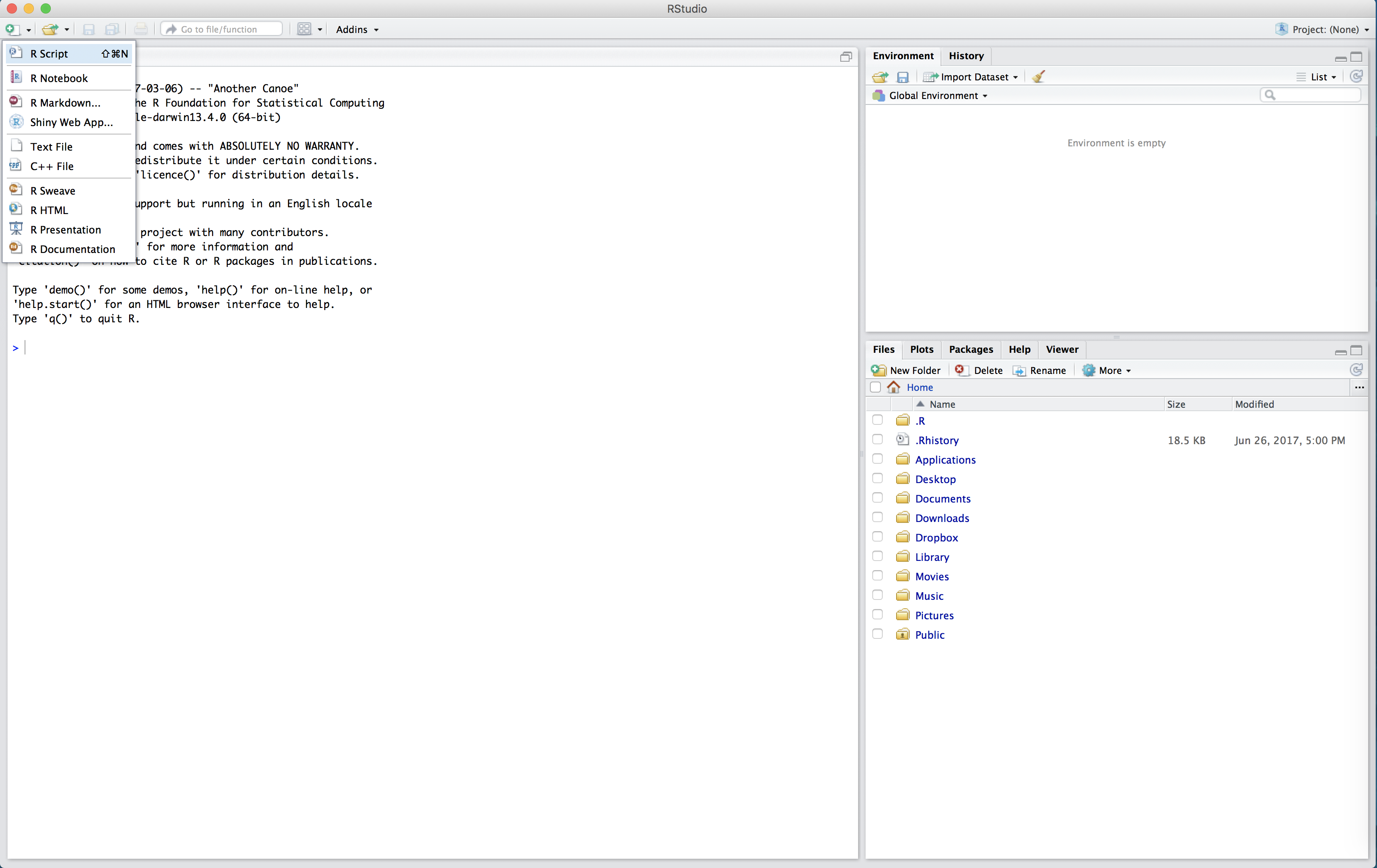
The untitled R Script will then appear in the top left hand box of R Studio.
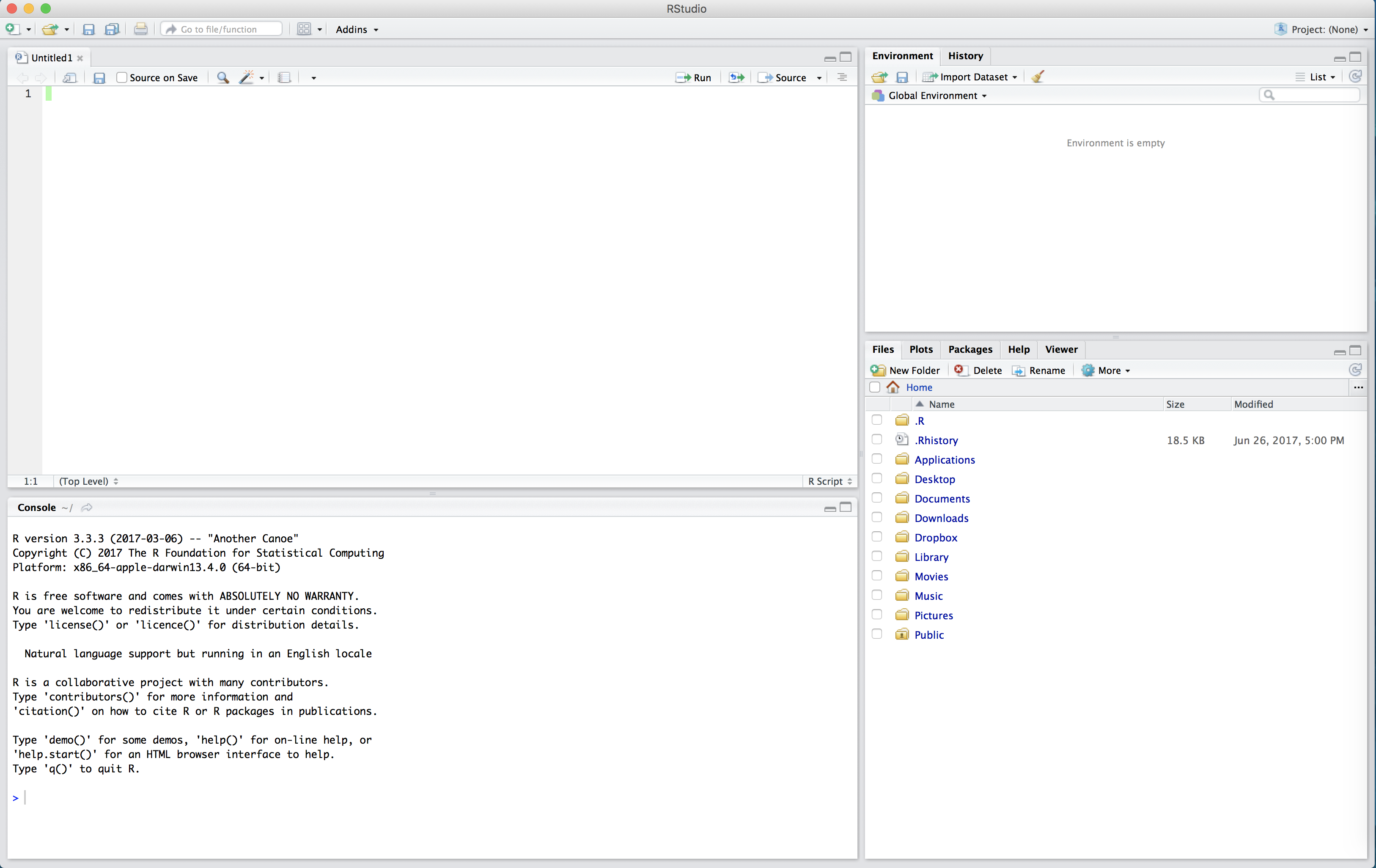
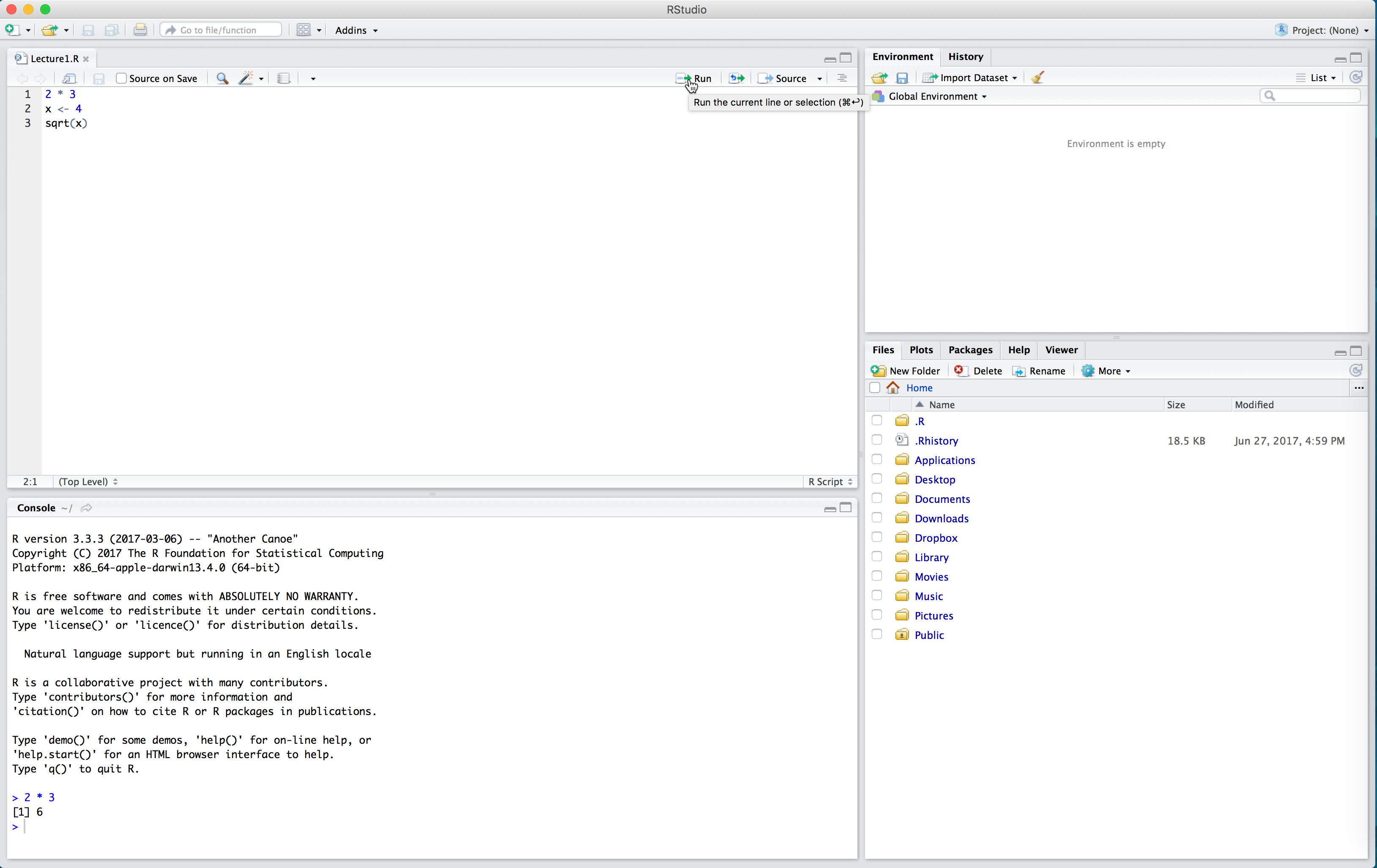
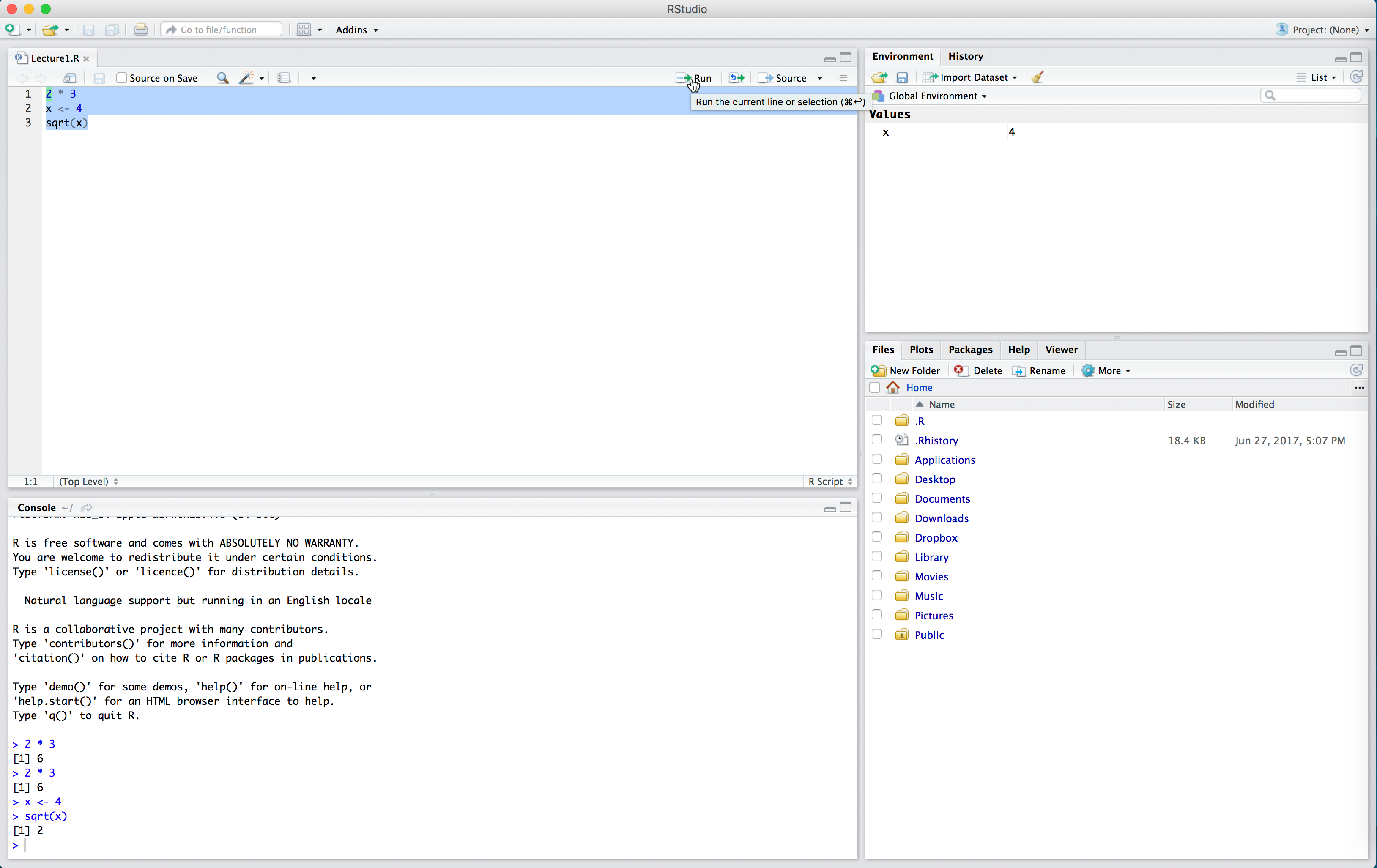
In the R Script, type the following:
2 * 3
x <- 4
sqrt(x)
Now our code is just sitting in the R Script. To run the code (that
is, evaluate it in the console) we click the “Run” button in the top
right of the script. This will run one line of code at a time -
whichever line the cursor is on. Place your cursor on the first line and
click “Run”. Observe how 2 * 3 now appears in the console,
as well as the output 6.
If we want to run multiple lines at once, we highlight them all and click “Run”.
Note in the above that we had to run x <- 4 before
sqrt(x). We need to define our variables first and run this
code in the console before performing calculations with those variables.
The console can’t “see” the script unless you run the code in the
script.
One very nice thing about RStudio’s script editor is that it will highlight syntax errors with a red squiggly line and a red cross in the sidebar. If you move your mouse over the line, a pop-up will appear that can help you diagnose the potential problem.
Another advantage of R scripts is that you can add comments to your code, which are preceded by the pound sign / hash sign #. Comments are useful because they allow you to explain what your code is doing. Throughout the rest of this course, we will be working almost exclusively with R scripts rather than directly entering commands into the console. For the sake of organization, you should save all of your scripts into the ‘scripts’ folder we created within the ‘Moneyball’ working directory.
Back to the NBA data
One huge advantage with working with R script is the ability to separate commands onto multiple lines. For instance, to add columns for FGP, FTP, and TPP to our tbl, we can write the following in our script window.
Notice how we have separated our command into multiple lines. This
makes our script much easier to read. While it seems a bit cumbersome to
write our code like this now, it will make our code much easier to read
when we start to string multiple manipulations together using the pipe
operator %>%, which we will meet in Lecture 3.