Problem Set X
Outline
Problem Set X is an additional, challenge problem set, designed to
accompany the material covered in Moneyball Academy. Topics covered
include advanced dplyr, merging datasets, simple regression, and ggplot2
graphing. You are strongly encouraged to attempt the problems for a
significant amount of time before looking at the answers for help. A
large portion of becoming an effective R-user is learning how to use
Google and StackOverflow to help you solve problems you’ve never
encountered before. You will be provided some direction and hints in the
problem descriptions. So, the solution code is by default “hidden”; to
check the solutions, click the “Code” buttons on the right of the page.
When looking through the solutions, if you don’t understand a function,
I encourage you to utilize the ?function command in the
Console (e.g. ?group_by). This will pull up the
corresponding R Documentation in the bottom right of your RStudio
window, under the “Help” section.
Suggested background reading:
Preparation
Load the following libraries, downloading if necessary: tidyverse, reshape2, ggrepel.
Download into your Moneyball/data folder and read into your environment the following datasets:
- statcast_2019.RData as
statcast_2019 - chadwick_register.csv as
chadwick_register - fangraphs_2019.csv as
fangraphs_2019- Data comes from this page, then clicking “Export Data” in the top right of the table. The Min PA filter on the FanGraphs leaderboard has been set to 0 for this download. FanGraphs is an excellent resource for advanced baseball statistics; if you are doing an MLB final project, I would recommend you use it to source your data.
- statcast_2019.RData as
The “playerid” column in
fangraphs_2019is FanGraphs’ own identification system. The corresponding MLB player id can be found as “key_mlbam” inchadwick_register. Useleft_join()to add the MLB player id tofangraphs_2019. This will enable us to later add FanGraphs statistics to additional data frames, merging on MLB player id.Remove rows from
statcast_2019with unrecorded attack regions using theis.na()function. Also remove rows describing games outside of the regular season, and save as a new data framenames. Reference the README.md in Box (the download location) to understand the features of the statcast dataset (this will also help you in future problems). Usingreframe(), reducenamesto a smaller, three column data frame, with each row containing a single batter, with their id, name, and number of pitches seen in the regular season. Consider what you will need to group by to achieve this result.
### Solution ###
library(tidyverse)
library(reshape2)
library(ggrepel)

load("data/statcast_2019.RData")
chadwick_register <- read_csv("data/chadwick_register.csv")
fangraphs_2019 <- read_csv("data/fangraphs_2019.csv") %>%
  left_join(select(chadwick_register, key_mlbam, key_fangraphs),
            by = c("playerid" = "key_fangraphs"))
# note the use of select within left_join(), keeping only the columns needed from chadwick_register

names <- statcast_2019 %>%
  filter(!is.na(attack_region), game_type == "Regular Season") %>%
  group_by(batterid) %>%
  reframe(batter_name = last(batter_name),
            pitches = n())
Swing Take Batter Summary
All of the following problems can be piped together, as one complete
block of code. Each instruction will correspond to an individual dplyr
function. You will begin with statcast_2019, and modify
from there. Save this new data frame as swtk19_summary. I
suggest you regularly open the data frame in the environment as you work
through the problems to check your progress.
Again, remove rows from
statcast_2019with unrecorded attack regions or describing games outside of the regular season.Write a conditional statement using
ifelse()to create a column “is_sw”, with “1” denoting if the batter swung at the pitch in question and “0” otherwise, filtering by the appropriate pitch descriptions. The%in%operator in R is useful to identify if an element belongs to a vector.Group the data by “batterid”, “attack_region”, and “is_sw”, in that order. Ask yourself, why is the order important?
Summarize the new groups, creating two columns: “n”, the number of observations in the group, and “rv”, the sum of the context neutral run value for that group, based on RE288. The
n()function returns the number of observations in the current group. Useround()to ensure “rv” is rounded to the second decimal place.swtk19_summaryshould now be a 6883 x 5 data frame.Ungroup. It’s good practice to always use
ungroup()after everygroup_by()to avoid potential unintended errors due to grouping, make pipes more readable by explicitly defining where the data is being operated on as groups.Combine “attack_region” and “is_sw”, such that there are now four total columns. Call this new, combined column “region”. Hint: explore the
unite()function, and set remove to be TRUE (this will remove the original columns you are combining).Use
melt()to convert your data frame into a form suitable for casting. Set your id variables to be “batterid” and “region”. Essentially, what melt does is transforms all remaining features (those not determined to be id variables) into two columns:variableandvalue. Variable will describe the column in reference (e.g. “n” or “rv”) and value will give the value for that variable corresponding to each particular id combination.Combine “region” and “variable” into one new column, “variable”, again using
melt(). Set remove = TRUE.Cast your molten data frame into a new, expanded data frame. Use the command
dcast(batterid ~ variable). Spend time here to understand the previous steps, 6-9, and consider circumstances in which you may wish to apply this approach. Check you understand whatHeart_1_rvorShadow_0_nmeans. Did you do the suggested reading?dcast()has left some missing values in the data frame. Replace all NAs with 0 using the commandreplace(is.na(.), 0).Add columns with the batter name and the number of pitches seen in 2019. Hint: join the previously created
namesdata frame.Add columns “Swing_Runs” (total run value when swinging), “Take_Runs” (total run value when taking), “Total_Runs” (total run value), and “TR_p100p” (total run value per 100 pitches). All of these columns should be rounded to the second decimal place.
Re-order the columns, such that they proceed in the following order (use the
everything()function withinselect()to minimize necessary order declarations): “batterid”, “batter_name”, “pitches”, “TR_p100p”, “Total_Runs”, “Swing_Runs”, “Take_Runs” “Chase_0_n”, “Chase_0_rv”, “Chase_1_n”, “Chase_1_rv”, “Heart_0_n”, “Heart_0_rv”, “Heart_1_n”, “Heart_1_rv”, “Shadow_0_n”, “Shadow_0_rv”, “Shadow_1_n”, “Shadow_1_rv”, “Waste_0_n”, “Waste_0_rv”, “Waste_1_n”, “Waste_1_rv”.Reduce the data frame to the 270 batters that saw the most pitches in the 2019 regular season. Hint: look at
top_n().Arrange the data frame in descending order by total run value per 100 pitches.
Add wOBA values for each batter. Hint: join the previously created
fangraphs_2019. Use select within the join command to keep only only the merge id column and wOBA.
### Solution ###
swtk19_summary <- statcast_2019 %>%
  filter(!is.na(attack_region), game_type == "Regular Season") %>%
  mutate(is_sw = ifelse(
    pitch_description %in% c("bunt_foul_tip", "foul", "foul_bunt", "foul_tip",
                             "hit_into_play", "hit_into_play_no_out",
                             "hit_into_play_score", "missed_bunt",
                             "swinging_strike", "swinging_strike_blocked"),
    1, 0)) %>%
  group_by(batterid, attack_region, is_sw) %>%
  reframe(n = n(),
            rv = round(sum(cnrv_288), 2)) %>%
  ungroup() %>%
  unite("region", attack_region:is_sw, remove = TRUE) %>%
  melt(id.vars = c("batterid", "region")) %>%
  unite("variable", region:variable, remove = TRUE) %>%
  dcast(batterid ~ variable) %>%
  replace(is.na(.), 0) %>%
  left_join(names, by = "batterid") %>%
  mutate(Swing_Runs = round(Heart_1_rv + Shadow_1_rv + Chase_1_rv + Waste_1_rv, 2),
         Take_Runs = round(Heart_0_rv + Shadow_0_rv + Chase_0_rv + Waste_0_rv, 2),
         Total_Runs = Swing_Runs + Take_Runs,
         TR_p100p = round(Total_Runs * 100 / pitches, 2)) %>%
  select(batterid, batter_name, pitches, TR_p100p, Total_Runs, Swing_Runs,
         Take_Runs, everything()) %>%
  top_n(270, pitches) %>%
  arrange(desc(TR_p100p)) %>%
  left_join(select(fangraphs_2019, key_mlbam, wOBA),
            by = c("batterid" = "key_mlbam"))
Interpreting Run Value
wOBA and Run Value
With your new
swtk19_summarydata frame, fit a linear regression usinglm(), with y = wOBA and x = TR_p100p.Add two new columns to
swtk19_summary: the predicted values based on your fit, usingpredict(), and the corresponding residuals.Graph a residual plot and double check your model is appropriate for the data.
Graph the relationship between total run value per 100 pitches and wOBA. Add your model regression line, and label the eight batters with the greatest residuals. Hint:
geom_label_text()can be used to text directly to the plot.geom_label_repel()draws a recentangle underneath the text, making it easier to read.What predictions for the 2020 season would you make about these eight batters, and why?
### Solution ###
fit <- lm(wOBA ~ TR_p100p, data = swtk19_summary)

swtk19_summary <- swtk19_summary %>%
  mutate(pred_wOBA = predict(fit),
         resid = pred_wOBA - wOBA)

# residual plot
#ggplot(swtk19_summary, aes(x = TR_p100p, y = resid)) +
#   geom_point()

ggplot(swtk19_summary, aes(x = TR_p100p, y = wOBA)) +
  geom_point(alpha = 0.5) +
  geom_smooth(method = "lm", formula = y ~ x) +
  geom_label_repel(data = top_n(swtk19_summary, 8, abs(resid)),
             aes(label = batter_name), min.segment.length = 0, size = 2,
             fontface = "bold") +
  theme_minimal() +
  ggtitle(label = "Comparing Run Value and wOBA of 2019 Batters",
          subtitle = ">500 pitches seen") +
  xlab("Context Neutral Run Value (per 100 pitches)") +
  theme(plot.title = element_text(size = 16, face = "bold", hjust = 0.5),
        plot.subtitle = element_text(size = 12, hjust = 0.5),
        axis.title.x = element_text(size = 12, face="bold"),
        axis.title.y = element_text(size = 12, face="bold"))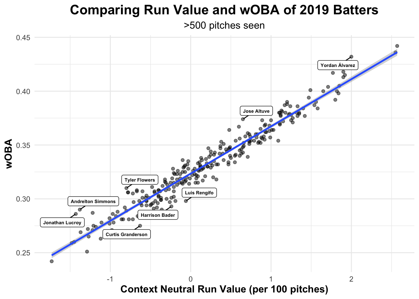
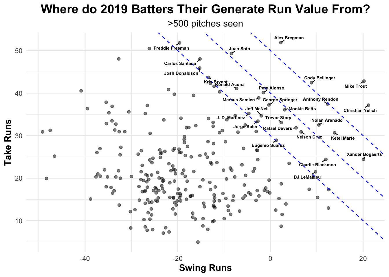
Run Value Generation
- Graph the relationship between run value generated from swings and
takes. Add guide lines using
geom_abline()to identify total run value benchmarks: 30, 40, and 50. Using a nestedfilter(), label players with >30 total run value.
### Solution ###
ggplot(swtk19_summary, aes(x = Swing_Runs, y = Take_Runs)) +
  geom_point(alpha = 0.5) +
  geom_abline(intercept = 50, slope = -1, linetype = "dashed", color = "blue") +
  geom_abline(intercept = 40, slope = -1, linetype = "dashed", color = "blue") +
  geom_abline(intercept = 30, slope = -1, linetype = "dashed", color = "blue") +
  geom_text_repel(data = filter(swtk19_summary, Total_Runs > 30),
                   aes(label = batter_name), min.segment.length = 0,
                   size = 2, fontface = "bold") +
  theme_minimal() +
  ggtitle(label = "Where do 2019 Batters Their Generate Run Value From?",
          subtitle = ">500 pitches seen") +
  xlab("Swing Runs") +
  ylab("Take Runs") +
  theme(plot.title = element_text(size = 16, face = "bold", hjust = 0.5),
        plot.subtitle = element_text(size = 12, hjust = 0.5),
        axis.title.x = element_text(size = 12, face="bold"),
        axis.title.y = element_text(size = 12, face="bold"))